In one experiment, F = {A, O, N, I} and T = {c, b, a, u, 1, 2, 3}. The parameters used per run are shown in the first column of
Table 4.24.
Table 4.24
Parameters for the density-classification task.
| |
GEP1 |
GEP2 |
| Number
of generations |
50 |
50 |
| Population
size |
30 |
50 |
| Number
of ICs |
25 |
100 |
| Function
set |
A O N
I |
I M |
| Terminal
set |
c b a
u 1 2 3 |
c b a
u 1 2 3 |
| Head
length |
17 |
7 |
| Number
of genes |
1 |
3 |
| Linking
function |
-- |
I |
| Chromosome
length |
52 |
39 |
| Mutation
rate |
0.038 |
0.051 |
| One-point
recombination rate |
0.5 |
0.7 |
| IS
transposition rate |
0.2 |
-- |
| IS
elements length |
1,2,3 |
-- |
| RIS
transposition rate |
0.1 |
-- |
| RIS
elements length |
1,2,3 |
-- |
The fitness was evaluated against a set of 25 unbiased ICs (i.e., ICs with equal probability of having a one or a zero at each cell). For this task, the fitness
fi of an individual program was a function of the number of ICs
n for which the system stabilized correctly to a configuration of all 0’s or 1’s after
2N time steps, and it was designed in order to privilege individuals capable of correctly classifying ICs both with a majority of 1’s and 0’s. Thus, if the system converged, in all cases, indiscriminately to a configuration of 1’s or 0’s, only one fitness point was attributed; if, in some cases, the system correctly converged either to a configuration of 0’s or 1’s,
fi = 2; in addition, rules converging to an alternated pattern of all 1’s and all 0’s were eliminated, as they are easily discovered and invade the populations halting the discovery of good rules; and finally, when an individual program could correctly classify ICs both with majorities of 1’s and 0’s, a bonus equal to the number of ICs
C was added to the number of correctly classified ICs, being in this case
fi = n + C. For instance, if a program correctly classified two ICs, one with a majority of 1’s and another with a majority of 0’s, it received 2 + 25 = 27 fitness points.
In this experiment a total of seven runs were made. In generation 27 of run 5, the following rule was discovered (only the K-expression is shown):
| 01234567890123456789012345678 |
|
|
OAIIAucONObAbIANIb1u23u3a12aa |
(4.39) |
This program (GEP1 rule) has an accuracy of 0.82513 tested over 100,000 unbiased ICs in a
149 X 298 lattice, thus better than the 0.824 of the GP rule tested in a
149 X 320 lattice (Juillé and Pollack
1998, Koza et al. 1999). Its rule table is shown in
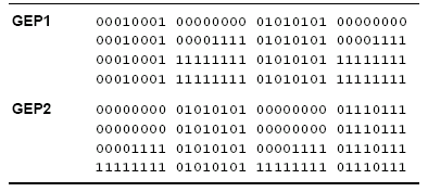
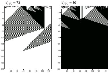
Table 4.25. Figure 4.15 shows two space-time diagrams for this new rule.
Table 4.25
Description of two rules discovered by GEP for the density-classification task. The output bits are given in lexicographic order starting with 0000000 and finishing with 1111111.

As a comparison, GP used populations of 51,200 individuals and 1,000 ICs for 51 generations (Koza et al.
1999), thus a total of 51,200 x 1,000 x 51 = 2,611,200,000 fitness evaluations were made, whereas GEP only made 30 x 25 x 50 = 37,500 fitness evaluations. Thus, at this task, gene expression programming not only surpasses GP by a factor of 69,632 but also discovered more and better rules than the GP technique.

Figure 4.15. Space-time diagrams describing the evolution of CA states for the
GEP1 rule. The number of 1’s in the IC (r0) is shown above each diagram. In both cases the CA converged correctly to a uniform pattern.
In another experiment a rule with an accuracy of 0.8255, thus slightly better than
GEP1, was discovered. Again, its performance was evaluated over 100,000 unbiased ICs in a
149 X 298 lattice. In this case F = {I, M}, and T was obviously the same. In this case, a total of 100 unbiased ICs and three-genic chromosomes with sub-ETs linked by IF were used. The parameters used per run are shown in the second column of
Table 4.24.
In this experiment, the fitness function was slightly modified by introducing a ranking system, in which individuals capable of correctly classifying between 2 ICs and 3/4 of the ICs received one bonus equal to
C; if correctly classified between 3/4 and 17/20 of the ICs received two bonus; and if correctly classified more than 17/20 of the ICs received three bonus. Also, in this experiment, individuals capable of correctly classifying only one kind of situation, although not indiscriminately, were differentiated and had a fitness equal to
n.
By generation 43 of run 10, the following rule (GEP2 rule) was discovered (the sub-ETs are linked with IF):
| 012345678901201234567890120123456789012 |
|
|
MIuua1113b21cMIM3au3b2233bM1MIacc1cb1aa |
(4.40) |
This program (GEP2 rule) has an accuracy of 0.8255 tested over 100,000 unbiased ICs in a
149 X 298 lattice, thus is better than the GEP1 rule and also better than the GP rule. Its rule table is shown in
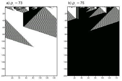
Table 4.25. Figure 4.16 shows two space-time diagrams for this new rule.

Figure 4.16. Space-time diagrams describing the evolution of CA states for the
GEP2 rule. The number of 1’s in the IC (r0) is shown above each diagram. In both cases the CA converged correctly to a uniform pattern.
In this chapter we have learned how to apply the basic gene expression algorithm to very different problem domains, introducing, along the way, a varied set of new tools that significantly enlarged the scope of the algorithm. These new tools include a facility for the manipulation of random numerical constants, a new class of comparison functions, bivariate basis polynomial functions, user defined functions, and automatically defined functions. In the
next chapter we are going to see how the elegant structure developed to manipulate random numerical constants in GEP can be further developed in order to allow the evolution of complex neural networks.
|