|
The objective of this section is to show how GEP can be used to model complex realities with high accuracy. The test function chosen is the following five parameter function:
|

|
(3.6) |
where a, b, c, d, and e are the independent variables.
Consider we are given a sampling of the numerical values from this function over 100 random points in the interval [-1,1] and we wanted to find a function fitting those values within 0.01% of the correct value. The fitness was evaluated by equation
3.3, being M = 100%. Thus, for
Ct = 100, fmax = 10000.
The domain of this problem suggests, besides the arithmetical functions, the use of
sqrt(x), log(x), 10x, sin(x),
cos(x) and tan(x) in the function set, which corresponds respectively to
Q, K, ~, S, C, and G. Thus, for this problem, F = {+, -, *, /, Q, K, ~, S, C, G} and
T consisted obviously of the independent variables {a,
b, c, d, e}.
For this problem, I chose 3-genic chromosomes encoding sub-ETs with a maximum of 19 nodes. The sub-ETs were posttranslationally linked by addition. The parameters used per run are summarized in
Table 5.
Table 5
Parameters for the problem of function finding on a five-dimensional parameter space.
| Number
of generations |
1000 |
| Population
size |
100 |
| Number
of fitness cases |
100 |
| Function
set |
+
- * / Q K ~ S C G |
| Gene
length |
19 |
| Number
of genes |
3 |
| Linking
function |
+ |
| Chromosome
length |
57 |
| Mutation
rate |
0.044 |
| One-point
recombination rate |
0.3 |
| Two-point
recombination rate |
0.3 |
| Gene
recombination rate |
0.1 |
| IS
transposition rate |
0.1 |
| IS
elements length |
1,2,3 |
| RIS
transposition rate |
0.1 |
| RIS
elements length |
1,2,3 |
| Gene
transposition rate |
0.1 |
| Selection
range |
100% |
| Precision |
0% |
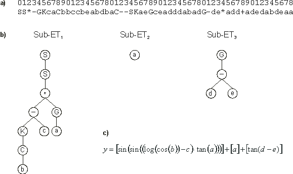
I used the software Automatic Problem Solver (APS) to model this function because it allows the easy optimization of intermediate solutions and the easy testing of the evolved models against a test set. In one run a very good solution, with an R-square of 0.9999913 evaluated over a test set of 200 random points, was found:
| 012345678901234567801234567890123456780123456789012345678 |
|
|
SS*-GKcaCbbccbeabdbaC--SKaeGceadddabadG-de*add+adedabdeaa |
(3.7) |
Its expression is shown in Figure 18.

Figure 18. Model evolved by GEP to fit the 5-parameter function
3.6. a) The model in Karva notation. b) The sub-ETs codified by each gene.
c) The corresponding mathematical expression after linking with addition (the contribution of each sub-ET is shown in square brackets).
This model is a very good approximation to the target function 3.6 as the high value for the R-square (almost 1) indicates. With APS we can further convert the evolved Karva programs into a more conventional computer program. For instance, the model
3.7 above can be automatically translated into the following C++ function:
|
double APSCfunction(double d[ ])
{
double dblTemp = 0;
dblTemp+=sin(sin(((log10(cos(d[1]))-d[2])*tan(d[0]))));
dblTemp += d[0];
dblTemp += tan((d[3]-d[4]));
return dblTemp;
} |
Note that the term encoded in the last gene matches exactly the second term of the
target function. However, a very unconventional and non-parsimonious alternative was found to express the first term of the target function. But the model evolved by GEP is, nonetheless, extremely accurate as the high value for the R-square indicates.
|
